Characteristic Curves

2-Terminal Devices

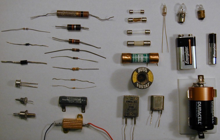
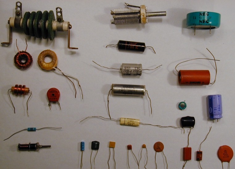
Many commonplace electrical components connect to the world through two terminals. From left to right above we have diodes, resistors, fuses, crystal oscillators, light bulbs and batteries. If we establish a voltage difference between the two wires, a current will usually flow. Generally the current will flow into (i.e., a positive current) the higher-voltage terminal and an equal current will flow out the low-voltage terminal. (The alternative to "current-in equals current-out" is a build-up of net charge inside the device. The electric force is simply too strong to sustain this. Even devices like capacitors and batteries which you may think of as "storing charge" in fact closely maintain charge neutrality.) Thus the relationship, I(V), between the applied voltage and the resulting current totally defines the device.

(Exceptions: some devices do depend on time: a discharged or charged battery, or temperature: a warm or cool filament in a light bulb... Perhaps temperature is the most common secondary parameter. Often a temperature coefficient, or "tempco", is specified to determine how a device behaves at different temperatures.) I say again: the relationship between applied voltage and resulting current -- the "IV characteristic curve" -- almost totally defines the device. This relationship can sometimes be usefully described with a formula; it can always be displayed as a graph of current (on the y-axis) vs. voltage (on the x-axis).

The most common example of this is the resistor, a two-terminal device with a linear relationship between current and voltage:

I = V/R

where R is the resistance, V is the voltage difference between the two terminals (V₂-V₁), and I is the current flowing into terminal 2. [Because it is potential difference that counts, often we take V₁=0 ("ground") so V₂ is the voltage difference, V. While the above may ease discussion, it in no way should suggest that in a real circuit V₁ must be at ground or that measurements can be made on the device by connecting terminal-1 to ground.] In a resistor R is a "constant" (of course subject to some tempco; years and use may also have some effect).

For any two-terminal device we can rearrange this relationship to define a "voltage dependent resistance":

R = V/I

although more often the "dynamic resistance"

r = dV/dI

is the useful concept. (Note that this dynamic resistance is the inverse of the slope of the IV curve.) The dynamic resistance is particularly useful if we seek small changes in current due to small changes in voltage near a particular "quiescent point" voltage V_Q. Taylor expanding the function I(V) in the vicinity of V_Q yields:

We can express this mathematical formula as a model equivalent circuit:

which simply displays that if the voltage drop across the device is changed by V the resulting change in current is exactly what would have been produced by a resistance r. Thus the dynamic resistance tells us how the device responds to changing voltages.

You may be under the impression the Ohm's "Law" is TRUE. While we can take various epistemological approaches to this, the most important point is that usually in electronics we're not so much looking for the TRUE as the useful. Real materials do not exactly follow Ohm's law...so what! The fact that many materials under normal conditions do approximately follow Ohm's law is what makes this a "law of electricity". That is to say, simple "models" of how devices behave normally and approximately are more valued than much more complex stories that might be more accurate. What is perhaps most valued is a sequence of increasingly accurate models allowing you to choose the needed level of accuracy and resulting burden of complexity. (Einstein: "Everything should be as simple as possible, but not simpler".) Note that we humans value simplicity as an aid to human understanding -- but computers rarely complain at being forced to do an additional million calculations.

Another aspect of my emphasis on simple models is an inversion of the revolutionary idea of interchangeable parts: The pistons coming off a GM engine assembly line are to a very high accuracy the same size so any can fill the cylinder. Alternatively we could design the engine so that more sloppily constructed pistons would still work. (Think piston rings.) In the electronics industry, available devices have a comparatively low level of reproducibility, so engineers have had to learn to make flexible (robust) designs. Given that individual electronic devices are far from identical, there is often no reason to use highly accurate models of the devices.

The upshot of all of this is that we're going to be looking for simple descriptions of our IV curves and we won't be put off if our model's predictions are a few percent off from measurements on a real device. While not the focus of these pages, additionally it is important to understand the physical basis of these models, so that, if possible, devices can be constructed with the characteristics we desire.

One of the first non-ohmic electronic devices invented was the diode. With a resistor if you reverse the voltage difference the current also reverses. (The two terminals on a resistor are interchangeable.) With a diode, voltage differences of one sign produce quite different results from the reversed sign. Perhaps the simplest model would be if V₂>V₁ the device behaves like a resistor, whereas V₂<V₁ no current flows:

The first diodes constructed worked by having the two terminals at different temperatures. One terminal (the "cathode") was heated to so high a temperature that electrons were easily pulled from it, allowing an electron flow from the cathode to the other terminal (called the "anode"). The anode was kept at room temperature; so its electrons stayed put and no current would flow in the reversed direction. Thus our first model is easy current flow in one direction; zero current flow in the other.

Since we understand the physics of the device, we can make an improved model. For electron flow through a "vacuum", it turns out that the current is not proportional to the voltage, rather the 3/2 power of voltage (Child's law):

I won't bother to explain what all the constants are in this expression, but do note that the basis of this law is understood. Devices with different characteristics could be designed by changing the the geometric constants of the device.

Real manufactured tubes do not exactly follow Child's Law. There is some current flow in the reverse direction ("cold emission") at large reverse voltages (see insert, about 10^-5 A reverse flow). For large positive voltages the measured current falls below that given by Child's law. At zero volts there is some positive (rather than zero) current flow. We could incorporate these additional complexities in our model of the device, if we really needed to.

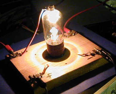
The above picture taken of the 3B24 vacuum tube while the above data was collected, shows the main problem: about 15 Watts of power required just to heat the cathode. The vacuum tube looks like an Edison light bulb (indeed, current flow in the vacuum tube is called the Edison Effect).

It was discovered you could make more efficient diodes (no heater required) out of semiconductors like silicon and germanium ("crystals"). Again the 0^th model is easy current flow in one direction, no current flow in the other. For silicon diodes the current flow remains "small", unless the forward voltage is greater than about 0.7 V. Thus our next model is easy current flow in one direction for forward voltages more than 0.7 V, otherwise no current flow. Again an understanding of how a semiconductor diode works shows that in simple cases there is an exponential relationship between voltage and current (Shockley's Law).

The aim of physics is to understand the basis of such a model, so for example, we want to understand the cause of the parameters I_s and V_T used in our models. Again, I won't bother to explain what the symbols mean in the below expression for I_s, but do note that the basis of Shockley's law is understood.

If you measure the IV curve for a real diode, you'll discover deviations from Shockley's law. Additional processes like the recombination current and high-level injection modify Shockley's law at low and high currents. Again, if we need a more accurate model these factors they can be included. But frankly the simplest model of a diode: that it is like a wire for current flow in one direction, and like a disconnect for current flow in the other, is what first comes to my mind when I need think about a circuit with diodes.

3-Terminal Devices

• NPN Bipolar transistors
• PNP Bipolar transistors
• n-channel field effect transistors (FETs)
• p-channel field effect transistors (FETs)
• n-channel MOSFETs
• p-channel MOSFETs

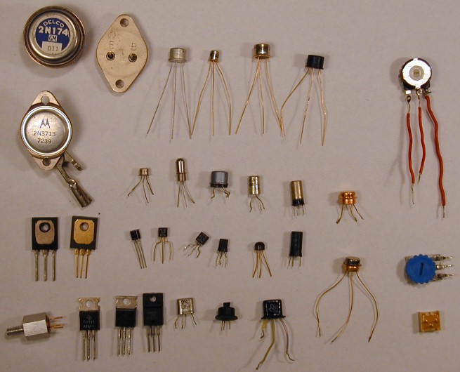
Many commonplace electrical components connect to the world through three terminals. Mostly I've displayed various types of transistors, but I've also included some potentiometers ("pots"). As above, for convenience we consider the voltage on one terminal to be zero (V₁=0). We then have four variables, two of which are independent: V₂, I₂, V₃, I₃. (Of course, device neutrality guarantees that the current flowing in: I₂+I₃ must flow out the first terminal.) For two terminal devices the current was just a function of the voltage, and the defining property was the IV-curve. For three terminals we have two independent quantities. Following the lead of the two-terminal discussion, we will take one of these to be V₂, but the other could reasonably be either V₃ or I₃. V₃ seems more natural, so let's begin there.

The next problem is how to display functions of two variables, like I₂(V₂,V₃). We could, of course, resort to a 3d perspective plot, with the height above the V₂-V₃ plane denoting I₂.

While such a plot might be evocative, we reject it as:

1. it would not be useful, because we can not easily extract numbers from such a perspective plot
2. it erroneously suggests some sort of equivalence between V₂ and V₃, whereas in fact for useful devices the two are designed to be quite different. (In future cases we'll use I₃ as the second variable so the two axes in the base plane will not even have the same units.)

and displaying the slices together.

(You should have seen similar plots displaying PVT relationships of gases in thermodynamics: PV curves for various fixed T ("isotherms") and "topographic" maps of mountains where the set of horizontal points at the same altitude are displayed as a curve.)

Practically speaking such plots are easy to produce: you just fix a value of V₃ and then vary V₂ collecting data points (V₂,I₂) to form your curve.

In the vicinity of a point Q, we can approximate changes in I₂ due to changes in V₂ and V₃ using a 2d Taylor's expansion:

(In our 2-terminal Taylor's expansion we were approximating the characteristic curves with a tangent line. In our 3-terminal Taylor's expansion we are approximating the characteristic surface with a tangent plane.)

We can play exactly the same game to express I₃(V₂,V₃), but I've never seen the results displayed a characteristic curves. Instead the y (admittance) parameters are sometimes provided.

We can express these mathematical formulae as a model equivalent circuit. I₂ increases in proportion to V₂ (exactly like a resistor) and there is an additional sink for current controlled by V₃: a source sinking a current equal to y₂₃V₃. (The current source parameter y₂₃ is often called the transconductance and denoted by g.)

where

r_out = 1/y₂₂

r_in = 1/y₃₃

g = y₂₃

In typical devices like FETs, y₃₂ is small and is usually neglected:

Often even greater model simplicity can be achieved: r_in (and sometimes r_out) are "large" enough to be neglected. In this simplest model, a FET is just a current source controlled by V₃.

The whole game can be re-played using I₃ as the other independent variable:

We can express these mathematical formulae as a model equivalent circuit. I₂ increases in proportion to V₂ (exactly like a resistor) and there is an additional sink for current controlled by I₃: a source sinking a current equal to h₂₃I₃. (The current source parameter h₂₃ is often called the current gain and denoted by .)

where

r_out = 1/h₂₂

r_in = h₃₃

= h₂₃

In typical devices like bipolar transistors, h₃₂ is small (ca. 10^-4) and is usually neglected:

In this simplest model, a bipolar transistor is just a "current multiplier" (i.e., a current source controlled by I₃) with input and output impedances.

AC Properties

I left out these important players because I was seeking simple models. Consideration of alternating current (AC) immediately introduces two additional parameters: frequency and phase shift. Most any circuit operating above the audio range (i.e., above 20 kHz) must include these additional complications. Here I will only comment that "stray capacitance" is the most important AC effect. More complex models of transistors would include little capacitors connecting each pair of terminals. At "low" frequencies the impedance of the capacitor:

Z_C=-i/C

is large and so the stray capacitors have little effect. However at higher frequencies these little capacitances are quite important.