Square Wells p.14

Spherical Square Wells

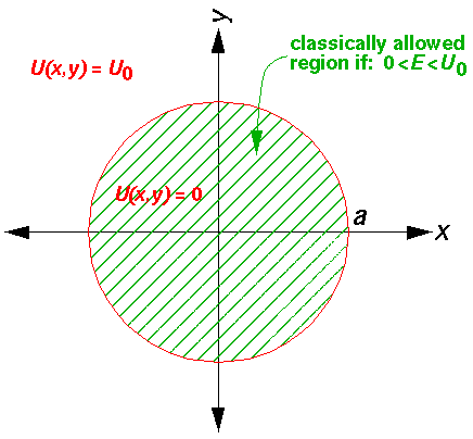
Since the problem is rotationally symmetric rather than square-symmetric, it makes more sense to use a coordinate system that reflects the symmetry in the problem. Hence, I'd like to solve this problem is spherical coordinates (r'--).

In spherical coordinates Schrödinger's equation reads:

Inside the well, where the potential is zero, U₀ would be set to zero.

The stuff in the square brackets (with the overall minus sign) is the (dimensionless) angular momentum squared operator: L'². The eigenfunctions of this operator are degenerate, so there is a choice to make in defining the basis states. In physics folks conventionally use the Y_lm, which are simultaneously eigenfunctions of both L'² and L'_z:

L'² Y_lm = l(l+1) Y_lm

L'_z Y_lm = m Y_lm

I direct your attention to the H-atom and SHM, where we have discussed a bit about these Y_lm.

Taking a as our length scale and ²/(2ma²) as our energy scale, we gain the dimensionless form

Seeking a solution where the dependence on r' factors from the dependence on angles ("separation of variables", =R(r') Y_lm(,)), we find:

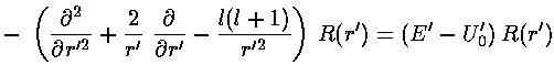
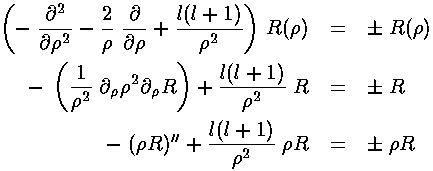
We will find it convenient to divide the above equation by E'-U₀', but we will need to pay attention as to the sign of (E'-U₀'). When (E'-U₀')>0 we are in a classically allowed region, and we expect the wavefunction to oscillate with a wavelength that depends on the particle's momentum... sin(kr) like solutions are to be expected. When (E'-U₀')<0 we are in a classically disallowed region, and we expect the wavefunction to exponentially decay...exp(-r) like solutions are to be expected. We'll handle both cases at the same time, sometimes by using ± signs where the top case (+ here) refers to a classically allowed region and the bottom case (- here) refers to a classically disallowed region. We substitute:

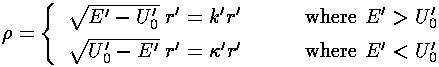
in our r' differential equation, producing a differential equation which I'll write in three equivalent forms:

As usual we'll have to work to solve the radial differential equation! Start by seeing how the the equation must work for large . If in the last equation we ignore the (very small) ^-2 term, we get the familiar oscillator differential equation. For E>U₀ we find:

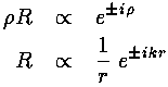
That is we see the expected oscillations as a function of r', but for large r' with ever smaller amplitude, because of the 1/r factor.

For E<U₀ we find:

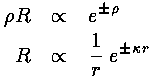
That is we see the exponential behavior as a function of r' expected in a classically disallowed region.

For small , the ^-2 term dominates and we can ignore the right hand side in comparison. If we try a power-law solution ⁿ

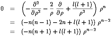
we find n=l.

Factoring out all the required behavior for small , we hope to find a simple power series for R:

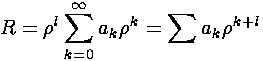
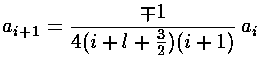
Plugging this in to the first R equation:

Or:

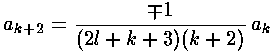
The result is a two term recursion relation (i.e., the result has just two as so, for example, given a₀ we can calculate a₂, from which we can calculate a₄, etc. until we're done.) Note that the the recursion relation connects even k to even k and since a₀ may not be zero (as the leading term ^l was needed to make the small differential equation work). Thus the series will have only even terms and we write our even k=2i, where i is an integer.

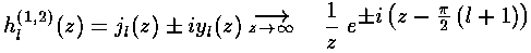
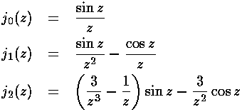
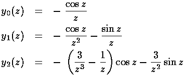
The series does not terminate; the result (for E>U₀) can be recognized as the spherical Bessel function j_l from the hypergeometric formula (₀F₁).

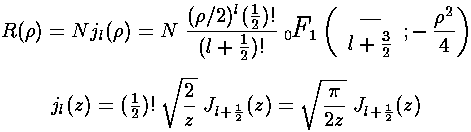
As shown above, spherical Bessel functions are related to normal Bessel functions with half-integral index.

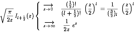
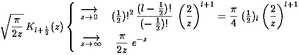
As we expect that a second order linear differential equation should have two independent solutions, we're only half way there. j_l is regular at =0, the other spherical Bessel function: y_l (also known as n_l) explodes at =0, and hence is not part of normalizable wavefunctions. Here are the basic large and small argument behaviors of j_l and y_l.

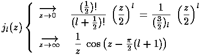
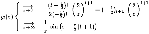
As we showed above, for large we expect oscillations like exp[±i]/. For small we expect ^l or ^-l-1, exactly as shown above. Here are some plots:

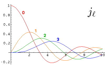
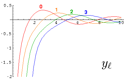
y and j are real functions and hence oscillate like sin and cos. If we want, we can put y and j together to produce something that for large oscillates like exp[±i]/. The results are related to Hankel functions and are also called spherical Bessel function of the third kind:

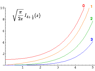
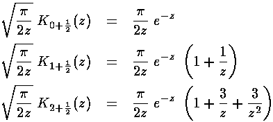
For E<U₀ we've found the exponentially rising modified spherical Bessel function related to I_l+½:

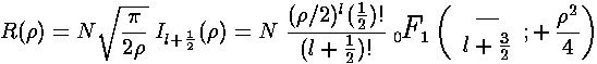
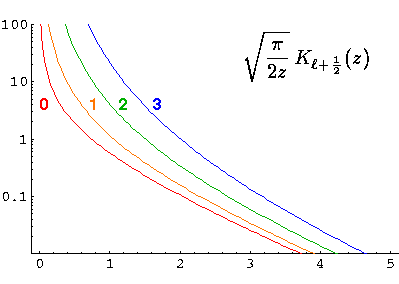
As above there is a second solution that is exponentially falling related to K_l+½:

The above expression may make spherical Bessel functions look as complex as the generic Bessel functions, but in fact, the spherical Bessel functions can be expressed in terms of well-known functions (whereas a generic Bessel function can not be so easily expressed):

Infinite Round Square-Well

j_l(k'r')=0 for r'=1

That is k' must be a zero of j_l. The energy of the wavefunction can then be calculated from

E'=k'²

Here is the overall solution:

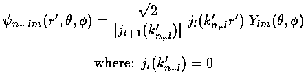
Because the angular dependence is "simple" we can usefully plot the wavefunction just as a function of r'. Here are "stacked wavefunction" plots for l=0,1,2:

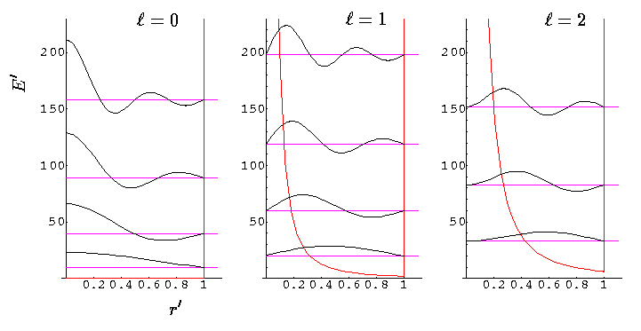
The red line is the classical "effective potential": l(l+1)/r'² (which is the "centrifugal potential") plus the infinite square well. Note that the centrifugal barrier excludes non-zero l wavefunctions from the origin.

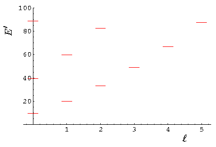
l,nr	root	E'
0,0	3.1	9.87
1,0	4.5	20.19
2,0	5.8	33.22
0,1	6.3	39.48
3,0	7.0	48.83
1,1	7.7	59.68
4,0	8.2	66.95
2,1	9.1	82.72
5,0	9.4	87.53
0,2	9.4	88.83

You should check each of the above roots on the above plots of j_j.

Here is what the set of energy levels looks like:

Next