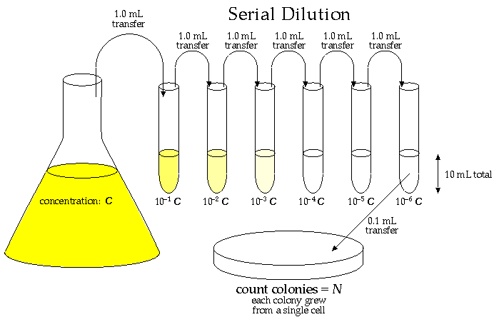
A primary characteristic of a culture of bacteria cells is its population density, C: the number of living cells per mL of solution. This is not an easy measurement to make! A culture would commonly have between a million (106) and a billion (109) "colony forming units" (cfu: i.e., viable cells) per mL, so personally counting the cells is out of the question. Furthermore it is hard to distinguish a living cell from a dead cell even in a microscope. The usual procedure is to dilute the solution by a huge factor so that in the end only a few (say 20-300) viable cells are sampled. The easiest way to count those viable cells is to let each one multiply producing a visible "colony" of millions of cells founded by just one cell from the culture. Thus we have the equation: one visible colony = one founding cell from the culture. (Note a possible source of error: careless technique in transferring can result in contamination: colonies founded by cells from the lab environment rather than the culture.)
So the first problem is to dilute the original culture by a factor of a million or so. This could be easily accomplished by taking 1 mL of the culture and mixing it with 999,999 mL of fluid medium. This is out of the question as 106 mL = 1000 L is about 4 garbage cans of solution. The alternative is serial dilutions: 6 dilutions in sequence each reducing the concentration by a factor of 10 (say by diluting 1 mL of the concentrate to 10 mL of solution).

Note a problem with this procedure: if you systematically transfer 5% (about a drop) too little or too much of the concentrate, then each dilution will be a little more or less than a factor of 10, and the final dilution would then be either
(9.5)6 = 0.74 × 10⁶
or
(10.5)6 = 1.34 × 10⁶
A series of 5% errors can result in a dilution error of 30% and a 30% error in the population density. Thus it is critical to accurately transfer the specified amounts!
Once we count the N colonies from the 0.1 mL of the most dilute tube, we know the concentration in that most dilute tube is:
concentration = (N cfu)/(0.1 mL) = 10 N cfu/mL
Before the dilution those N bacteria were in a volume of only: (0.1 mL) × 10-6
Thus the original concentration C is given by:
C = (N cfu)/(0.1 mL × 10-6 ) = 107 × N cfu/mL
Note that if you plate out another 0.1 mL aliquot of the most dilute solution, your pipet is unlikely to capture exactly the same number of bacteria cells it did the first time. The expected variation in the count (given by Poisson statistics) is the square root of the count: N½. Thus we could write our final formula for the culture concentration as:
C = 107 × (N ± N½ ) cfu/mL
For example if N=100, we'd have:
C = 107 × (100 ± 10) cfu/mL = (109 ± 108) cfu/mL
Another way of estimating the uncertainty in C would be to repeat the whole process lots of times and take as the final value for C the average of the Cs, with an uncertainty given by the standard deviation of the mean. In fact this is what the FDA requires for many of its mandated tests.
I assume I've convinced you that counting bacteria cells is not easy! It is also a slow process: you must wait 24 hours for the colonies on the plate to grow into colonies large enough to see and count. Thus there is a real need for a quick and easy way to measure population density.
Remark: In the end of this process we're going to be entering big numbers, like 108, for population density into the computer. How is this done? First off, note a simple solution: just switch units.
108 cfu/mL = 102× 106 cfu/mL = 100 Mcfu/mL
where we have made use of a Système International multiplier: Mega=M=million=106. If we enter all our numbers in the unit Mcfu/mL we'll only have simple numbers to enter. Note the general formula:
C = 10 × (N ± N½ ) Mcfu/mL
Since C is exactly proportional to N you could also do all our plotting and fitting with N and only later multiply by 10 (if you want Mcfu/mL) or 107 (if you want cfu/mL).
The other approach is to use the "E" (or "e") notation for entering big or small numbers into computers:
6.023 × 1023 = 6.023E23
108 = 1 × 108 = 1e8
600 nm = 600 × 10-9 m = 600e-9 m = 6e-7 m
1 µm = 10-6 m = 1 × 10⁻⁶ m = 1e-6 m
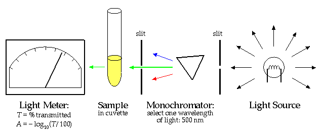
The "Beer-Lambert Law" states that there is a linear relationship between the concentration of a solution and the "absorbance", A.
[X] = k A
Thus a measurement of A with a spectrophotometer and knowledge of the proportionality constant k allows you to calculate the concentration, [X]. (The proportionality constant can itself be calculated by finding the absorbance of a solution with known concentration.)
Why can't this same trick work to find the concentration of bacteria cells in a culture? If you've worked with cultures you've seen that as the bacteria multiply the solution becomes "cloudy". The cloudier the solution, the higher the population density of the cells. Cloudy is precisely the right word: the bacteria cells act just like the water droplets in a cloud; they scatter the light. The more scatters in the way of the light beam, the less light that gets through. However while light scattering (redirecting light in a different direction) and light absorption (total removal of light from the beam) both have the effect of diminishing the light that makes it directly through the sample, scattering of light is quantitatively different. Repeated scattering within the sample can take light that had been directed out of the beam, back into the beam. Furthermore, depending on the precise geometry of the spectrophotometer's light meter, the light meter may record slightly scattered light as transmitted light. The upshot of all this is that the linear relationship of Beer-Lambert can only be expected to apply to dilute solutions where multiple scattering is rare. There is no general formula relating concentration of scatters and measured A, because the measured A depends both on the solution being measured and the internal construction of the particular spectrophotometer.
Lacking a fundamental formula, our remaining option is calibration. Measure both the population density (using the above long method) and the A (easy!) of several different cultures (or the same culture as it grows). Plot this data and draw a smooth curve that best matches the measured points. Recall that the measured population will have an uncertainty, so there is no reason to expect that the smooth curve goes exactly through each experimentally measured point, rather the smooth curve needs only come "close" to the expect range. Once you have found your smooth curve if you measure the A of the culture, you can use the curve to find the population density that would produce that A. Once you have found the calibration curve, you need not repeat the long colony-counting procedure to determine C.
Some Vocabulary: Mixtures of fine particles in a fluid (bacteria in growth medium; water droplets in air) are called suspensions rather than solutions. Turbid is the adjective used to describe the cloudiness of suspensions. Since the word "absorbance" does not suggest light scattering, I'll use the alternative general term "optical density" (OD) when referring to the measured "absorbance" of a suspension.
Our first job is decide which variable to put on the x axis and which on the y axis.
One rule is to put the low error quantity on the x axis. Since C and OD have different units we must compare them in terms of "percent error": the ratio of the variation in a value to the value.
For a typical colony-count like N=100, the variation in C due to counting is 10%=N½/N.
Its hard to judge the accuracy of the OD read from the dial of a Spectronic 20D. The manufacturer's specifications suggests accuracies of a few %T which would be approximately ±10% for OD in the useful range of .1 to 1. On the other hand, the readings of a Spectronic 20D are quite reproducible; the manufacturer's specifications are not random errors, but rather systematic calibration errors. We can think of the Spectronic 20D's calibration as being folded into the calibration for C. Thus what we seek is a formula relating the number displayed on the Spectronic 20D and C; we don't really care if the number displayed on the Spectronic 20D is precisely absorbance. In this sense there is little uncertainty in the measured "OD".
So, depending on how you are thinking of things, the error in OD is either comparable to the error in C or much less.
Another rule is to put the "controlling" variable on the x-axis. In this case, concentration causes "absorption" rather than the other way around, so this would suggest putting concentration on the x axis.
However, our aim in this process is to find a formula calculating concentration from OD, so OD must go on the x-axis.
Here is our data:
| OD | N | N½ | C (Mcfu/mL) |
|---|---|---|---|
| 0.071 | 12 | 3.5 | 120 ± 35 |
| 0.156 | 28 | 5.3 | 280 ± 53 |
| 0.236 | 34 | 5.8 | 340 ± 58 |
| 0.300 | 54 | 7.3 | 540 ± 73 |
| 0.363 | 70 | 8.4 | 700 ± 84 |
| 0.448 | 75 | 8.7 | 750 ± 87 |
| 0.568 | 97 | 9.8 | 970 ± 98 |
| 0.701 | 98 | 9.9 | 980 ± 99 |
Here is a result of fitting a smooth curve through these points:
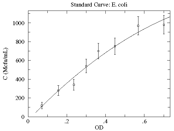
The "smooth curve" is a curve that mostly passes through the
error bars (which have a size denoted by  ).
Where the error
bars are large, the
deviation from the curve (denoted by
 , shown in blue below) can also be large.
(The data points deviate from the curve by different amounts;
 is the deviation of the first point from the
curve;
  is the deviation of the second point from the
curve;
  is displayed below.)
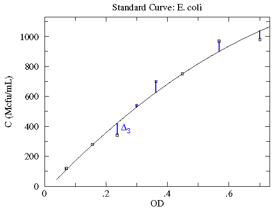
What counts is the relative size of the deviation and the error bar.
"Good" points have a small (less than 1) ratio of deviation
( ) to
error (
 ); "Bad" points have a ratio of deviation to error larger than one,
and hence the curve fails to go through the error bar (as in
the third data point). On average a good fit will have as
many unusually large deviations as unusually small deviations, that is,
on average the ratio of deviation to error will be about 1. (Of course,
in a perfect fit the curve will go right through every data point:
zero deviation.)
  is defined as the sum of the square
of each data point's ratio of deviation to error:

On average we expect each term in the sum to be about
1 so the total ( ) should be about
equal the number of data points. However by selecting
a fitting-curve with as many adjustable parameters as data points,
you can usually force the curve to exactly hit every data point:
a perfect fit but probably of no significance. Approximately
speaking, each adjustable parameter of the curve should allow you
to exactly hit one data point. The number of "effective"
data points, i.e., those that could not be automatically hit
by the curve, is called the number of "degrees of freedom".
degrees of freedom (d.f.)= number of data points - number of adjustable parameters
Below our eight data points are exactly hit by a polynomial with eight adjustable parameters, but no one would think that the actual relationship is this bizarre
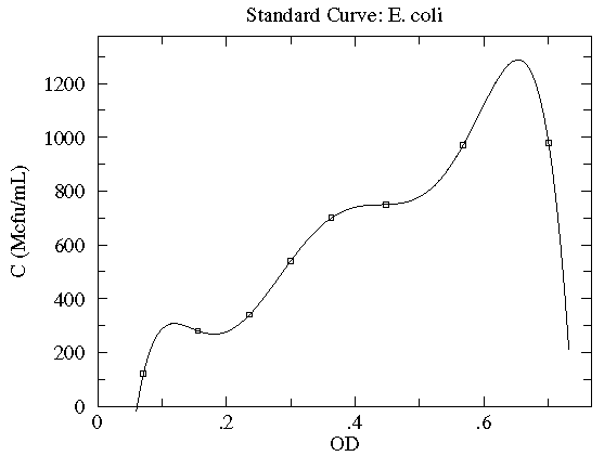
Thus we can make  zero by selecting a curve
that twists and turns to hit every point. Clearly it is
a useless process to fit a curve exactly through inexact data. We
want a curve with as few twists and turns as possible that comes
near (or better yet: inside) each error bar. We focus then on
the
  per degree of freedom:
reduced chi-square=
 /(d.f.)
This number should be expect to be near one. (If it is less than one, we have an unexpectedly good fit; If it is much greater than one, the curve is missing too many data points to be believed.)
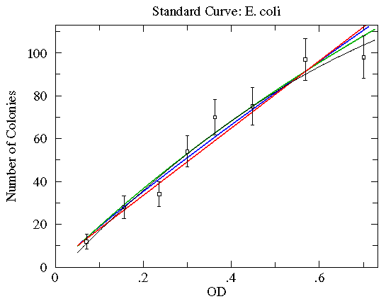
| Curve | color | reduced | Parameter Values | ||
|---|---|---|---|---|---|
| a | b | c | |||
| Linear y=a+bx | red | 0.93 | 2.11 | 157 | |
| Power y=a xb | blue | 0.85 | 153 | 0.911 | |
| Inverse X & Y 1/y=a+b/x | green | 0.77 | 0.00207 | 0.00504 | |
| Quadratic y=a+bx+cx2 | black | 0.73 | -3.7 | 215 | -88 |
These functions have essentially the same values over the region covered by the data; any of them would make a fine choice.
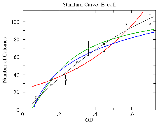
Here are some function choices which do not make good fits (reduced chi-square of about 2½ to 5; green=Arrhenius, blue=Natural Log, red=Exponential). The other WAPP function choices are even worse.
In order to do chi-square fitting you need: