WAPP⁺: Parameter Errors

Obviously parameter values "near" that minimum have essentially the same value of , and hence are nearly as likely as the "best fit" values. However, at sufficiently great distances from the "best fit" values, the resulting value of is unlikely. The standard commonly used for an "unlikely" value of is one more than the minimum value. Thus to determine range of possible parameter values, we need to find the region where:

χ²(A,B) ≤ χ²_min + 1

Consider first the simple case of a linear fit:

f (x) = A + B x

where does not depend on A or B (i.e., no x-errors). Thus, if we expand out the terms in the definition:

and then bring together terms with the same powers of A and B, we find a simple quadratic form in A and B:

= a A² + b AB + c B² + d A + e B + f

The set of (A,B) parameters that produce a fixed value of χ² is an ellipse. A collection of such constant-χ² curves is like a topographic map of the function χ²(A,B); the desired set of "likely" values of A and B is the valley in χ²(A,B) bounded by the ellipse:

χ²(A,B) = χ²_min + 1

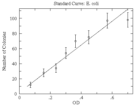
Consider the data set first discussed here:

OD N δN 0.071 12 3.5 0.156 28 5.3 0.236 34 5.8 0.300 54 7.3 0.363 70 8.4 0.448 75 8.7 0.568 97 9.8 0.701 98 9.9

WAPP⁺ gives the following report:

An analysis of the data submitted indicates that a function of the form:
--Linear-- y=A+Bx
can fit the 8 data points with a reduced chi-squared of 0.93

                FIT
 PARAMETER     VALUE        ERROR
   A =          2.120        3.5    
   B =          156.7        12.    
 
 NO x-errors

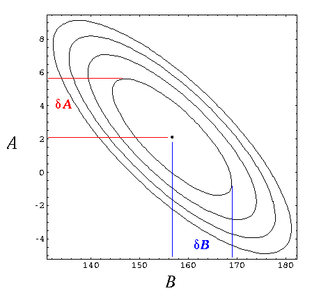
Below is the resulting countour plot of χ². The minimum value of χ² is 5.58 and it occurs at

(B,A)=(156.7,2.12)

(denoted as the central black dot in the below plot). The ellipses are the constant χ² curves for Δχ²=1,2,3,4.

Notice, for example, that line with a slope higher than the best-fit value (larger B) is made possible by shifting the entire curve down i.e., a smaller y-intercept (smaller A), for example (169,-1). The extreme value of B with Δχ²=1 is about 169 and is denoted with the rightmost blue line. Similarly, the extreme value of A with Δχ²=1 is about 5.7 and is denoted with the highest red line. These extreme values define the range of likely parameter values, so we find graphically (and consistently with the more exact calculations of WAPP⁺):

A =2.1 ± 3.6

B =157 ± 12

(In this simple case the extreme values below the best fit values must be symmetrically located, because of the symmetry of the error ellipse...hence "±". In a more general case---i.e., one with x-errors---this symmetry would only be approximate.)

Summary: WAPP⁺ determines parameter errors from the extremes of the Δχ²=1 curve. Further mathematical details may be found here. As discussed below and here, if the minimum reduced χ² is not near one, WAPP⁺ renormalizes your errors to achieve reduced χ²=1 before calculating parameter errors.

Warning: Systematic Errors Not Included

Warning2: Systematic Errors Often Dominate

Example

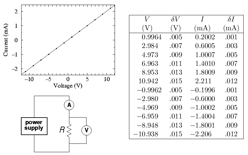
Fitting the expected linear relationship (V=R I), WAPP⁺ reports:

An analysis of the data submitted indicates that a function of the form:
--Linear-- y=A+Bx
can fit the 12 data points with a reduced chi-squared of 0.11

This chi-squared is "small." If the data and error bars were plotted the fitted curve would lie inside almost all the error bars, i.e., the data show smaller fluctuations from the fitted curve than would be expected given errors you reported. Perhaps the measurement error is systematic rather than random. In any case the reported parameter errors have been reduced to match the level of fluctuation seen in the data.

                FIT
 PARAMETER     VALUE        ERROR
   A =        -0.9820E-03   0.14E-02
   B =          4.968       0.16E-02

V_actual = α + βV_measured

where α is small and β ≈ 1; the manufacturer's specifications really are reporting that α and β deviate from a perfect calibration, not that there is random variation in the readings. Using the manufacturer's specifications (essentially δV/V=0.001 and δI/I=0.005) we would expect any resistance calculated by V/I to have a relative error of sqrt(.1^2+.5^2)=.51% (i.e., an absolute error of ±.025 kΩ for this resistor). WAPP⁺, on the other hand, reports an error 16 times smaller. Part of the reported error reduction is due to WAPP⁺'s "renormalization" of errors in view of the impossibly small reduced χ²...WAPP⁺ is saying

the only situation in which my calculated parameter errors make sense is if the measurement errors are random, and if the error in this data is random, it must be much smaller than was reported...small enough to get a reduced χ² near one. In that case the parameter errors are as shown

Lesson: Fitting programs can badly underestimate errors when systematic calibration errors are present.

Comment: If a high precision resistance measurement is required there is no substitute for making sure that when the DMM reads 1.00000 V the actual voltage is also 1.00000 V. Calibration services exist to periodically (typically annually) check that the meters read true.

If the maximum applied voltage in the resistance experiment is changed from ±10 V to ±40 V a new problem arises. The reduced χ² for a linear fit balloons by a factor of about 50. The problem here is that our simple model for the resistor V=R I (where R is a constant) ignores the dependence of resistance on temperature. At the extremes of voltage (±40 V) about 1/3 W of heat is being dumped into the resistor: it will not remain at room temperature. If we modify the model equation to include power's influence on temperature and hence on resistance, say:

V = B(1 + β I²) I

(where fitting constant B represents the room temperature resistance and β is a factor allowing the electrical power dissipated in the resistor to influence that resistance), we return to the (too small) value of reduced χ² seen with linear fits to lower voltage data. You might guess that the solution to this "problem" is to always use the most accurate model of the system under study. However it is known that that resistance of resistors depends on pressure, magnetic field, ambient radiation, and its history of exposure to these quantities. Very commonly we simply don't care about things at this level of detail and seek the fewest possible parameters to "adequately" describe the system. A resistor subjected to extremes of voltage does not actually have a resistance. Nevertheless that single number does go a long way in describing the resistor. With luck, the fit parameters of a too-simple model have some resemblance to reality. In the case of a single resistance, the resulting value is something of an average of the high and low temperature resistances. In these circumstances it is unlikely that the reported error in a fit parameter has any significant connection to reality (like the difference between the high and low temperature resistances) since the error will depend on the number of data points used.

Lesson: We are always fitting less-than-perfect theories to less-than-perfect data. The meaning of the resulting parameters (and certainly the error in those parameters) is never immediately clear: judgment is almost always required.

The quote often attributed to Einstein: "things should be made as simple as possible, but not simpler" I hope makes clear that part of art of physics is to recognize the fruitful simplifications.