
where k is a parameter in the first Brillouin zone of reciprocal space. Physically k is the crystal momentum, that shows the behavior of the wavefunction between real lattice cells, and uk shows the probability density in every cell.
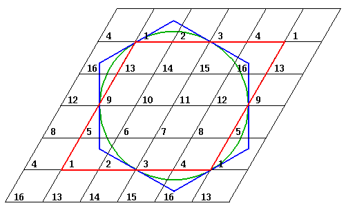
This problem lacks an algebraic answer...we hare going to have to solve this equation by computer approximation. We begin by griding: breaking up our unit cell into smaller pieces. We hope that the value of the wavefunction at these grid points will well-represent the wavefunction even between the grid points. I've included in the below diagram our red rhombus which we use to tile real space. The centered circle of attraction is shown in green. In case you wondered what a honey-comb of hexagons would look like instead of the tiling of rhombuses, I've included a centered blue hexagon.

Notice that I've force the function to be periodic.
We can approximate the derivative w.r.t. x by the
difference between neighboring points along the x axis.
Thus the derivative w.r.t. x at grid point 2 is approximately
the difference between the values at grid points 3 and 1 divided by
 x between grid points 3 and 1:

where h is the grid-rhombus side, so
 x=2h.
In the above griding h=¼.
Approximating the derivative w.r.t. y is a bit more of a problem because none of the neighboring grid points just differ in y. If we average u at grid points 5 and 6 we should approximate u directly up from grid point 2; similarly the average of grid points 14 and 15 approximates u directly below grid point 2. The difference between these two averages should give us the derivative w.r.t. y:

Approximating the Laplacian at 2, is a bit tricky. Recall that the Laplacian tells you how much the function differs from its average value on surrounding points. With a little bit of work (see the Mathematica file) one can show:

Thus if our differential equation is to be satisfied at 2 we must have:

The above is a big ugly equation. (I hope you scrolled to see it all.) The most important feature is that it is a linear equation in the ui. Thus is could be rewritten:

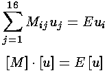
There is nothing special about grid point 2; it is a similar story or each grid point so:

Notice we are left with an eigenequation for the 16×16 matrix M. Don't forget that the elements of M depend on the parameter k, so the eigenvalues E(k) are are desired band structure.
It is a useful to test your understanding of this grid technique! Below find the core matrices for the Laplacian, and the derivatives. Please check out a few rows and see that they make sense to you.
Laplacian = (2/3)*
-6  1  0  1  1  0  0  1  0  0  0  0  1  1  0  0
 1 -6  1  0  1  1  0  0  0  0  0  0  0  1  1  0
 0  1 -6  1  0  1  1  0  0  0  0  0  0  0  1  1
 1  0  1 -6  0  0  1  1  0  0  0  0  1  0  0  1
 1  1  0  0 -6  1  0  1  1  0  0  1  0  0  0  0
 0  1  1  0  1 -6  1  0  1  1  0  0  0  0  0  0
 0  0  1  1  0  1 -6  1  0  1  1  0  0  0  0  0
 1  0  0  1  1  0  1 -6  0  0  1  1  0  0  0  0
 0  0  0  0  1  1  0  0 -6  1  0  1  1  0  0  1
 0  0  0  0  0  1  1  0  1 -6  1  0  1  1  0  0
 0  0  0  0  0  0  1  1  0  1 -6  1  0  1  1  0
 0  0  0  0  1  0  0  1  1  0  1 -6  0  0  1  1
 1  0  0  1  0  0  0  0  1  1  0  0 -6  1  0  1
 1  1  0  0  0  0  0  0  0  1  1  0  1 -6  1  0
 0  1  1  0  0  0  0  0  0  0  1  1  0  1 -6  1
 0  0  1  1  0  0  0  0  1  0  0  1  1  0  1 -6

dx = (1/2)*
 0  1  0 -1  0  0  0  0  0  0  0  0  0  0  0  0
-1  0  1  0  0  0  0  0  0  0  0  0  0  0  0  0
 0 -1  0  1  0  0  0  0  0  0  0  0  0  0  0  0
 1  0 -1  0  0  0  0  0  0  0  0  0  0  0  0  0
 0  0  0  0  0  1  0 -1  0  0  0  0  0  0  0  0
 0  0  0  0 -1  0  1  0  0  0  0  0  0  0  0  0
 0  0  0  0  0 -1  0  1  0  0  0  0  0  0  0  0
 0  0  0  0  1  0 -1  0  0  0  0  0  0  0  0  0
 0  0  0  0  0  0  0  0  0  1  0 -1  0  0  0  0
 0  0  0  0  0  0  0  0 -1  0  1  0  0  0  0  0
 0  0  0  0  0  0  0  0  0 -1  0  1  0  0  0  0
 0  0  0  0  0  0  0  0  1  0 -1  0  0  0  0  0
 0  0  0  0  0  0  0  0  0  0  0  0  0  1  0 -1
 0  0  0  0  0  0  0  0  0  0  0  0 -1  0  1  0
 0  0  0  0  0  0  0  0  0  0  0  0  0 -1  0  1
 0  0  0  0  0  0  0  0  0  0  0  0  1  0 -1  0

dy = 1/(2*sqrt(3)) *
 0  0  0  0  1  0  0  1  0  0  0  0 -1 -1  0  0
 0  0  0  0  1  1  0  0  0  0  0  0  0 -1 -1  0
 0  0  0  0  0  1  1  0  0  0  0  0  0  0 -1 -1
 0  0  0  0  0  0  1  1  0  0  0  0 -1  0  0 -1
-1 -1  0  0  0  0  0  0  1  0  0  1  0  0  0  0
 0 -1 -1  0  0  0  0  0  1  1  0  0  0  0  0  0
 0  0 -1 -1  0  0  0  0  0  1  1  0  0  0  0  0
-1  0  0 -1  0  0  0  0  0  0  1  1  0  0  0  0
 0  0  0  0 -1 -1  0  0  0  0  0  0  1  0  0  1
 0  0  0  0  0 -1 -1  0  0  0  0  0  1  1  0  0
 0  0  0  0  0  0 -1 -1  0  0  0  0  0  1  1  0
 0  0  0  0 -1  0  0 -1  0  0  0  0  0  0  1  1
 1  0  0  1  0  0  0  0 -1 -1  0  0  0  0  0  0
 1  1  0  0  0  0  0  0  0 -1 -1  0  0  0  0  0
 0  1  1  0  0  0  0  0  0  0 -1 -1  0  0  0  0
 0  0  1  1  0  0  0  0 -1  0  0 -1  0  0  0  0
These may look like big matrices, but in the calculations on the following pages I've refined the griding a factor of two to make 64×64 matrices. Mathematica can crank right through problems of that scale. We occasionally further refine the grid to h=1/16 (i.e., 256×256 matrices)... this slows the calculation down considerably. [I'd worry about a further refinement, unless the problem is coded in a faster language like fortran.]