Oscillations show up throughout physics. From simple spring systems in mechanics to atomic bonds in quantum physics to bridges blowing the wind, physical systems often act like oscillators when they are displaced from stable equilibria.
In this experiment you will observe the behavior of a simple sort of oscillator: the torsion pendulum. In general a torsion pendulum is an object that has oscillations which are due to rotations about some axis through the object. This apparatus allows for exploring both damped oscillations and forced oscillations.
Note that angular frequency (ω in rad/s) and frequency (f in Hz.) are not the same. Most the equations below concern ω, in many cases it is easier to measure f.
In the damped case, the torque balance for the torsion pendulum yields the differential equation:
|
| (1) |
where J is the moment of inertia of the pendulum, b is the damping coefficient, c is the restoring torque constant, and θ is the angle of rotation [?]. This equation can be rewritten in the standard form [?]:
 | (2) |
where the damping constant is β =  and the natural frequency is ω0 =
  . The general solution to this
differential equations is:
. The general solution to this
differential equations is:
![[ √----- √ -----]
θ(t) = e-βtA e β2-ω20t + A e- β2- ω20t ,
1 2](torsion_pendulum4x.png) | (3) |
with three different types of solutions possible depending on the relationships between ω0 and β.
In the underdamped case (β < ω0):
 | (4) |
with the oscillation frequency ω1 =  , initial amplitude θ0, and phase γ.
In the critically damped case (β = ω0):
 | (5) |
In the overdamped case (β > ω0):
![θ(t) = e-βt[A1eω2t + A2e-ω2t],](torsion_pendulum8x.png) | (6) |
where ω2 =  .
.
For the forced oscillation case, an external torque is added to Equation 1:
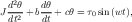 | (7) |
where ω is the driving frequency and τ0 is the driving torque [?]. The general solution to the differential equation is the sum of the homogeneous solutions (which are the solutions to the damped case above) plus a particular solution. The particular solution has the form:
 | (8) |
with
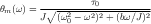 | (9) |
In this case the resonance frequency is ωr =  and the phase shift between the pendulum and the
external oscillator is:
and the phase shift between the pendulum and the
external oscillator is:
 | (10) |
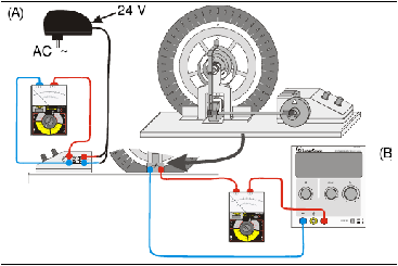
In this experiment you will use the torsion pendulum, the power supply for the driving motor, a low voltage power supply for the eddy current damper, two digital multimeters, and a stop watch.
Figure 1 shows the torsion pendulum and associated electronics. The motor which is used to force the pendulum (which will only be used in the second half of the experiment) is shown on the left of the diagram. The eddy current damping device is shown on the bottom of the diagram.
The instructions below assume that you will collect data bye eye, but you can also use video capture to collect the data. The torsion pendulum data can also be taken by video capture, either using the camera attached to the Raspberry Pi in PE 132, or with your own cell phone. Then the files can be analyzed using Tracker (https://www.cabrillo.edu/~dbrown/tracker/).
Set up the pendulum with a white background behind it, and light it well. Log into the Raspberry Pi, and run the video capture software using a command like the one below:
raspivid -w 640 -h 480 -fps 5 -t 10000 -o pend_jc1.h264
The command is raspivid, the -w and-h options set the width and height of the video, th -fps sets the frame rate in frame per second, -t sets the length of the video in microseconds, and -o sets the name of the output h264 video file.
After creating the video files, you can transfer them to the Linux computer yalow, by copying them to /var/yalow. Once copied there, they will show up on yalow under /backup. From there, you will need to change the files into mp4 format, so that Tracker can use them:
avconv -i pend_jc1.h264 -c copy -r 5 pend_jc1.mp4
This command changes the h264 file into an mp4 file, which tracker can deal with. The command avconv can do fancier things like change the frame rate or size of the image as well. (A similar command called ffmpeg is available on the regular Linux computers.)
Tracker is currently just installed on yalow. To run it log into yalow from the console, or remotely using ssh:
ssh -Y physics@yalow
Then either find Tracker in the menu, or from a terminal type:
/opt/tracker/tracker.sh
To use Tracker, you can use the fine documentation under Help, particularly Getting Started. Here’s an even briefer overview:
First, setup the torsion pendulum apparatus, with the forcing motor turned off and play with it to get an idea of how it works [?].
With damping magnet turned off, find the natural frequency by measuring the period of the torsion pendulum. You will probably get better results if you use the time it takes the pendulum to oscillate 10 or 20 times to find the period. Note that even with the current off, friction does cause some damping of the pendulum. So the motion is not quite simple harmonic motion.
Pick a small value of the damping current (0.1 A < I < 0.3 A) and determine the damping constant. To do this first measure the period several times. Then start the pendulum from its furthest rotation point and measure θmax after each period. If you have difficulty taking the θmax measurements, you may need to try again. If using video capture, you can just take one long video at a given damping current, and collect all of the needed information from that video.
Plot θmax versus time. Your plot should look like a decreasing exponential. Fit your data to find a value for the damping constant, β.
Repeat this process for a higher value of the damping current (0.3 A < I < 0.6 A).
Increase the damping current until the system only completes one oscillation after you let it go from its furthest rotation point, so the pendulum only crosses 0 once and then approaches 0 from the negative side. Find the oscillation time for this case by taking several measurements and taking the average.
Then increase the current until the pendulum approaches 0 from the positive side, but never crosses 0. This is the critically damped case. Use several measurements for the time it takes the pendulum to reach the equilibrium in this case.
Now use the critically damped case to get an estimate of the damping constant, β, in this case. Find the damping constant from equation 5 by measuring the time that it takes the pendulum to reach some fixed θ, say θ0 ∕10, after releasing it from its furthest rotation point. Note that in this case you can assume B = 0 and that A = θ(t = 0) in equation 5. Since ω0 = β in the critically damped case, you can use this β to get estimates of the damping coefficient, b, and the restoring torque, c. Recall that J = 3.0 ± 0.1 kg⋅m2.
Now put the current at a higher value (but remember to keep it under 2.0 A). This is an overdamped case. Find the oscillation time in this case.
First, setup the torsion pendulum apparatus with the forcing motor turned on and play with it to get an idea of how it works [?]. Note that you may have to give the pendulum an initial displacement to get it moving, but that initial motion will damp out, leaving only the forced oscillations.
Find the resonance frequency of the torsion pendulum from a amplitude (θmax) versus driving frequency plot for the torsion pendulum. In this section, you will need to decide on a procedure yourself, based on what you know about the device and resonance curves. While you are doing taking data, be sure to note the phase behavior of the driver and the oscillator before, at, and past resonance. You should find resonance curves and frequencies for three different brake (damping) currents (~ 0 A, ~ 0.4 A, and 0.8 A). Also, find the damping constant for those three cases.