We have found the following wavefunctions for the infinite spherical square well:
with energy E'=k'2.
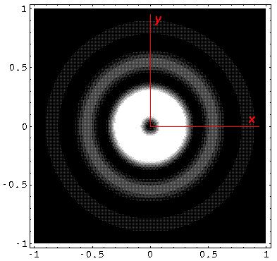
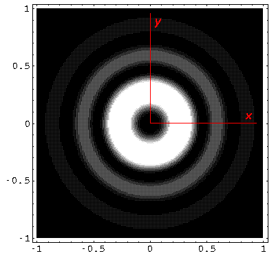
We looked at 1D plots of these wavefunctions, but what do the probability densities look like in space? The l=0 (s-wave) wavefunctions are spherically symmetric, so the 1D plots show the successive shells around the center.
If l isn't zero the
probability densities for these wavefunctions are not spherically
symmetric. However the probability densities (but not the wavefunctions
themselves)
are independent of  ("cylindrically symmetric" for a cylinder
whose axis is aligned with the z axis) so we only need to concern
ourselves with their dependence on
("cylindrically symmetric" for a cylinder
whose axis is aligned with the z axis) so we only need to concern
ourselves with their dependence on  and r (i.e.,
for example the x-z plane).
(The exp(im) dependence in the wavefunction cancels out in
and r (i.e.,
for example the x-z plane).
(The exp(im) dependence in the wavefunction cancels out in
 *.)
The probability density for +m and -m
are identical (since
Yl,-m=(-1)mY*l,m;
the difference is only which way the particle is going
around the z axis. Note that except for l=0 the wavefunction goes to
zero as you approach the origin; the larger the value of l the faster you
go to zero. Note that unless m=0 the wavefunction
is zero on the z axis; again larger |m| means a more
disallowed z axis. For the largest possible |m| (i.e.,
m=±l) the probability is largely near the
x-y plane. Finally, there are always nr radial
nodes (zeros) [not counting the origin or well edge].
*.)
The probability density for +m and -m
are identical (since
Yl,-m=(-1)mY*l,m;
the difference is only which way the particle is going
around the z axis. Note that except for l=0 the wavefunction goes to
zero as you approach the origin; the larger the value of l the faster you
go to zero. Note that unless m=0 the wavefunction
is zero on the z axis; again larger |m| means a more
disallowed z axis. For the largest possible |m| (i.e.,
m=±l) the probability is largely near the
x-y plane. Finally, there are always nr radial
nodes (zeros) [not counting the origin or well edge].
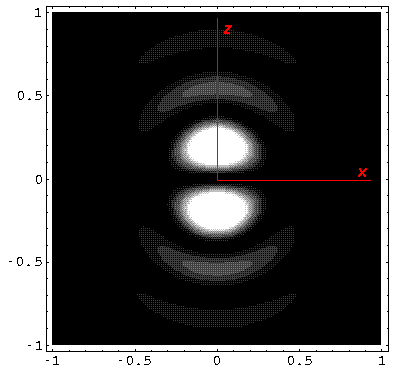
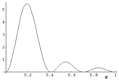
Note from the 1D plots that the probability density is high near the origin. In fact in the contour plots the central region is "over exposed", i.e., in order to show the details on the large outer lobes, I chose a maximum contour (pure white) that was well below the the first peak's height.
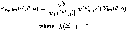
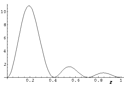
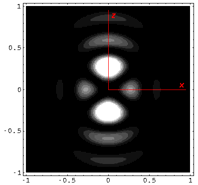
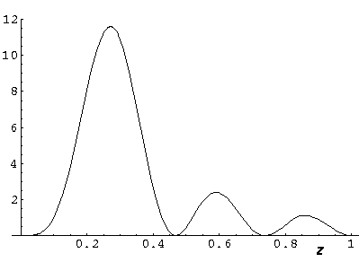
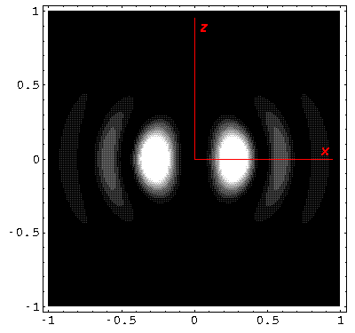
Below we plot the probability density for nr=2, l=1 ("p" wave) for m=0,1. For several of these plots the probability density is also plotted along a particular line.
Note that chemists call this the pz orbital. There is a node on the plane z=0. One can use linear combinations of the l=1 m=±1 wavefunctions to produce orbitals identical to pz, except located around the x- (called px) and y- (called py) axes (i.e., with nodal planes x=0 and y=0).
Note that the probability is somewhat confined to the z=0 plane (i.e.,
the x-y plane)
Here is what the probability density looks like in that plane; like all
of these solutions it's symmetric
Below we plot the probability density for nr=2, l=2 ("d" wave) for m=0,1,2. For several of these plots the probability density is also plotted along a particular line.
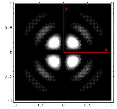
Note that the probability is mostly confined to the z=0 plane (i.e.,
the x-y plane)
Here is what the probability density looks like in that plane; like all
of these solutions its symmetric
The display "problem" of high probability densities near the origin is commonly
"solved" by plotting r rather then .
As we explained earlier the result of this is to produce
WKB-like wavefunctions.
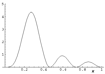
Here is what r looks like for nr=10,
l=0 E'=1194:
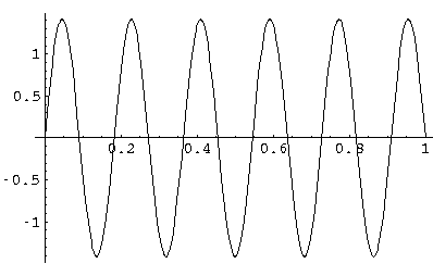
This is exactly a sine wave; If you were surprised look back at the
differential equation for ( R)...for l=0
it is the famous differential equation:
R)...for l=0
it is the famous differential equation:
f'' = -f.
Note that for this l=0 solution,
is spherically symmetric and has 10 nodal spheres. Don't be fooled by the above
plot: the probability density oscillations are not of uniform height.
Probability density is highest near the origin.
Here is what it like for nr=5, l=10 E'=1080
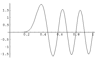
Note the exclusion of this high l wavefunction from the origin.
(Don't forget that this radial solution must be matched with various Y10m; none is spherically symmetric.)
Finally note that in producing the above "Ylm" solutions, we have
produced complex rather than real wavefunctions....
that factor of exp(im). This factor
cancels out of our *
probability density (so the probability density is -symmetric),
but if we were to look at just the real part of
we would find oscillation as a function of
in addition to its oscillations in .
Oscillation indicates momentum, so these
solutions have angular momentum...in fact m angular momentum in the "z" direction (i.e., perpendicular to the
plane) and a total angular momentum squared of
2l(l+1). One can
easily produce real valued wavefunctions (like px,
dxy, etc. discussed previously) but these seemly simpler
functions in fact turn out to be more difficult to calculate with.
angular momentum in the "z" direction (i.e., perpendicular to the
plane) and a total angular momentum squared of
2l(l+1). One can
easily produce real valued wavefunctions (like px,
dxy, etc. discussed previously) but these seemly simpler
functions in fact turn out to be more difficult to calculate with.