We have found the following wavefunction for our 3-d oscillator:
with energy E'=4nr+2l+3.
What do these wavefunctions look like?
If l=0 the wavefunctions are spherically symmetric.
If l>0,
the probability densities for these wavefunctions (but not the wavefunctions
themselves)
are independent of  ("cylindrically symmetric" for a cylinder
whose axis is aligned with the z axis) so we only need to concern
ourselves with their dependence on
("cylindrically symmetric" for a cylinder
whose axis is aligned with the z axis) so we only need to concern
ourselves with their dependence on  and r (i.e.,
for example the x-z plane).
(The exp(im) dependence in the wavefunction cancels out in
and r (i.e.,
for example the x-z plane).
(The exp(im) dependence in the wavefunction cancels out in
 *.)
The probability density for +m and -m
are identical (since
Yl,-m=(-1)mY*l,m );
the difference is only which way the particle is going
around the z axis. Note that except for l=0 the wavefunction goes to
zero as you approach the origin; the larger the value of l the faster
goes to zero. Note that unless m=0 the wavefunction
is zero on the z axis; again larger |m| means a more
disallowed z axis. For the largest possible |m| (i.e.,
m=±l) the probability is largely near the
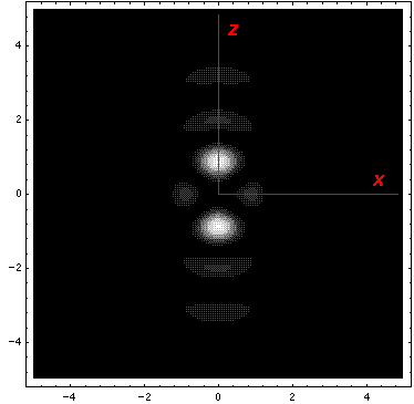
x-y plane. Finally, there are always nr radial
nodes (zeros) [not counting the origin].
*.)
The probability density for +m and -m
are identical (since
Yl,-m=(-1)mY*l,m );
the difference is only which way the particle is going
around the z axis. Note that except for l=0 the wavefunction goes to
zero as you approach the origin; the larger the value of l the faster
goes to zero. Note that unless m=0 the wavefunction
is zero on the z axis; again larger |m| means a more
disallowed z axis. For the largest possible |m| (i.e.,
m=±l) the probability is largely near the
x-y plane. Finally, there are always nr radial
nodes (zeros) [not counting the origin].
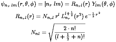
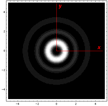
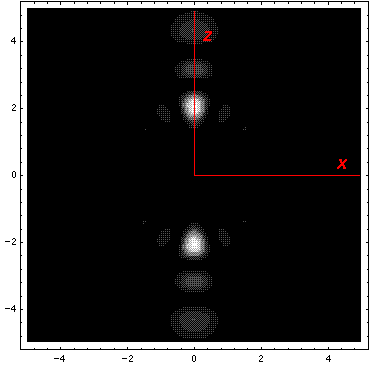
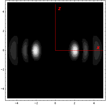
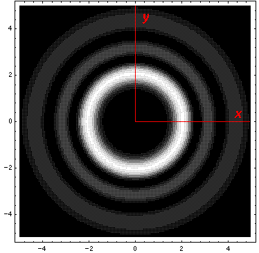
Below we plot the probability density for nr=2, l=2 ("d" wave) for m=0,1,2. For several of these plots the probability density is also plotted along a particular line.
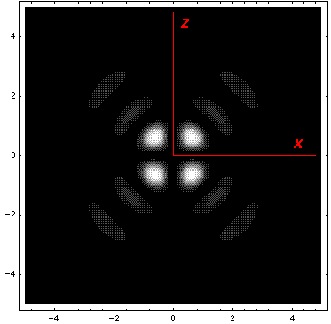
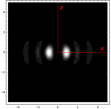
Note that the probability is mostly confined to the z=0 plane (i.e.,
the x-y plane)
Here is what the probability density looks like in that plane; like all
of these solutions it is symmetric
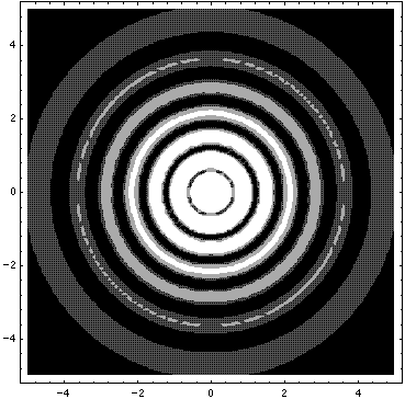
All the the above solutions have E'=15. Here is a collection of solutions with E'=27.

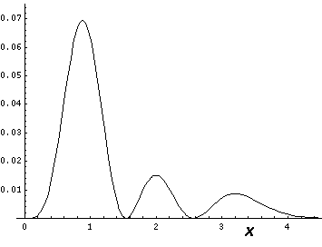
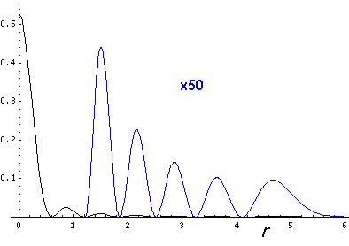
This l=0 solution is spherically symmetric, so all planes going through the origin have the same probability density. For this particular case there is such a large difference between the probability density at the origin and for the last few oscillations near the edge of the classically allowed region, that I have had to "stretch" the scales. In the case of the density plot, contours are spaced equally in logarithm (here a factor of 2 separates adjacent contours) rather than arithmetically (constant differences) spaced; in the case of the plot of probability density vs r, I've included a "50×" magnified plot of the large r probability density.
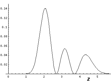
Because the angular dependence is "simple" we can usefully plot the wavefunction just as a function of r. Here are "stacked wavefunction" plots for l=0,1,3:
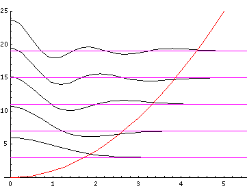
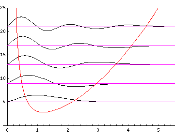
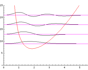
The red line is the classical "effective potential"= l(l+1)/r2+r2 which includes the "centrifugal barrier" l(l+1)/r2 for a particle with l total angular momentum (essentially) l. Because of the centrifugal barrier, non-zero l wavefunctions are excluded from the origin.