SHM p.11
Seeing QM Oscillation: 2-d
It is quite easy to produce visible x-y oscillation:
just find the sum of y wavefunctions that oscillates
in y (working exactly as in the 1-d case) and
find the sum of x wavefunctions that oscillates
in x and multiply them together. Most of the probability
will be in a lump at a particular (moving) (x,y).
To build up an orbiting probability packet, we must use
wavefunctions with minimal inward/outward motion (i.e., nr=0)
and large angular momentum (i.e., large positive m). We will use
as our model wavefunction a function that is localized in
 but with lots of oscillation in
  ,
i.e., exp[-100
 2+200i
 ]).
Our |nr=0, m> wavefunctions do, of course,
depend on r: basically restricting the wavefunction to
r near m½, i.e., the bottom of the
effective potential. But for small variations in m, this will be much
the same r. Thus we focus on localizing in
  .
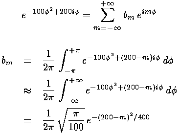
We start by straightforward Fourier expansion of our model wavefunction
in terms of exp(im
 ), the
  behavior of the |nr=0, m> wavefunctions.

Using these same bm to expand our wavefunction should
achieve similar localization in  while localization in
r' is automatic for large m, nr=0
wavefunctions. In practice one can't sum over an infinity of m,
but the equation for bm shows that bm
is large only for m near 200 (so we restrict our sum to between
180 and 220).

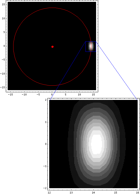
Below is displayed the resulting lump of probability for t'=0.

We need not display similar plots for other times because the equation
for  shows that plot for any other time are
identical to the above except rotated by 2t' radians. Thus
the lump will make one complete revolution in a period of

Next
 but with lots of oscillation in
  ,
i.e., exp[-100
 2+200i
 ]).
Our |nr=0, m> wavefunctions do, of course,
depend on r: basically restricting the wavefunction to
r near m½, i.e., the bottom of the
effective potential. But for small variations in m, this will be much
the same r. Thus we focus on localizing in
  .
We start by straightforward Fourier expansion of our model wavefunction
in terms of exp(im
 ), the
  behavior of the |nr=0, m> wavefunctions.


 shows that plot for any other time are
identical to the above except rotated by 2t' radians. Thus
the lump will make one complete revolution in a period of
