SHM p.3

We have found a length scale l and an energy scale e, now we use these to transform Schrödinger's equation into dimensionless form. We make a dimensionless position: x'=x/l and a dimensionless energy: E'=E/e and plug those into Schrödinger's equation.

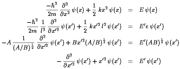
The next step is to determine the large x' behavior of , and then factor it out of . The term x'² obviously grows with x'; one of the other terms must cancel it. Since E' is constant it can't help, so there must be an approximate cancellation of the first two terms for large x'. exp(-x'²/2) has the desired property: its second derivate (for large x') is approximately x'²× itself. Thus we seek a solution of the form: =H(x') exp(-x'²/2). (This is "without loss of generality" [wolog], i.e., for any there is such an H(x'). We hope, however, that finding H(x') will be easier than finding directly.)

If we now try to write H as a polynomial:

we can plug the polynomial form into the differential equation:

The result is a two term recursion relation (i.e., the result has just two as so, for example, given a₀ we can calculate a₂, from which we can calculate a₄, etc. until we're done.) Note that the the recursion relation connects even k to even k and odd k to odd k. Thus the polynomials will have only even or odd terms.

It turns out that the polynomial must end if the wavefunction is to be normalizable. One can show that the non-terminating sum gets at least as big as exp(+x'²), so instead of going to zero for large x' gets big like: exp(+x'²/2). The only way the sum can end is if the numerator of the recursion relation is zero, i.e., if E'=1+2n then a_n+2=0 (and hence all further as are zero).

Note that if we had tried for a polynomial solution for itself (rather than factoring out the exp(-x'²/2) first), we would get an (unsolvable) three term recursion relation.

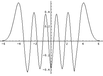
The polynomials we have found are called Hermite polynomials (see for example, Abramowitz & Stegun, §22 p. 771 or Szegö Ch.V). Below is a plot of a Hermite polynomial (H₁₀(x)=-30240 + 302400 x² - 403200 x⁴ + 161280 x⁶ - 23040 x⁸ + 1024 x¹⁰) ) from x=-4 to 4 and x=-2 to 2

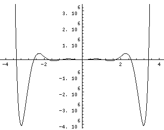
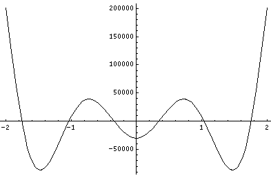
Note that H₁₀(x) is an even function with ten real roots, and like any polynomial it becomes huge for large |x|.

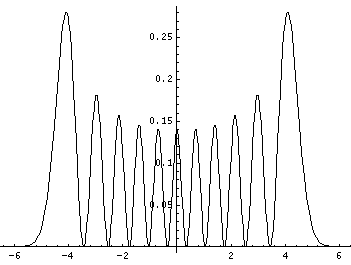
The corresponding position probability density and wavefunction (i.e., with the exp(-x'²/2) factor) are plotted below.

n E'
0 1
1 3
2 5
3 7
4 9
5 11

n	E'
0	1
1	3
2	5
3	7
4	9
5	11

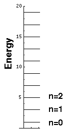
Notice that we have a discrete set of energy levels, i.e., energy is quantized and the particle can have only the above energies. Quantum mechanics says energies between these levels will not be seen in nature. A discrete set of levels is expected if the particle is confined to a region.

Notice that the energy levels are exactly evenly spaced. (Energy spacing (i.e., differences) are quite important as (1) that is what is observed in emitted photon energies and (2) that is what is related to the classical period.)