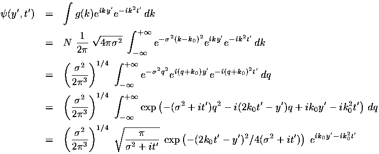
We have found a particular solution to the time dependent Schrödinger's equation:
This solution represents a superposition of single-energy solutions making a lump of probability that moves
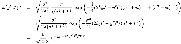
In dimensionless units the velocity of the wave-packet is 2k0. If we convert this to normal quantities we find:
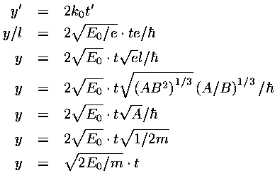
i.e., the wave-packet moves with the velocity expected for a particle with that (average) energy.
In the above the primed quantities are dimensionless versions of the usual variables (e.g., y vs y'). I'll now drop the primes, but everything is to be considered the dimensionless quantity.
There is lots to be learned by carefully examining graphs
of this solution. It is hard, however, to plot  in the usual way on the "y" axis, since
takes on complex (rather than just real) values. My solution here is
to plot both the real part of (which shows oscillations)
and the absolute value of . You can estimate the
imaginary part of by looking at the difference between
|| and Re().
in the usual way on the "y" axis, since
takes on complex (rather than just real) values. My solution here is
to plot both the real part of (which shows oscillations)
and the absolute value of . You can estimate the
imaginary part of by looking at the difference between
|| and Re().
The variable k0 determines the typical "wavelength" of the oscillations:
k0 = 2 /
/
so short wavelength corresponds to large k0. In the below, note that when k0=6 the wavelength is about 1, and when k0=3 the wavelength is about 2. Recall that the fourier transform g(k) shows which simple waves make up the wave-packet. Thus the peak of g(k) is at k0.
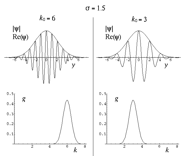
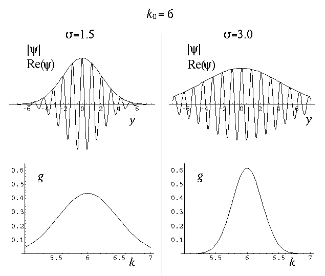
The variable  determines the initial width of the
lump of probability. At the same time (because of Heisenberg's Uncertainty)
it determines the range of speeds (momentums, energies) that contribute
significantly to the superposition. Large spatial extent means a reduced
range of wavelengths to make up the packet. Thus while the peak of g(k)
is at k0, the width of the peak is determined by
. Large-sized wave-packets have a large
and a narrow peak in g(k). (If the spatial extent of the wavefunction
is large the waves that make up the packet must have quite similar
wavelengths, otherwise those waves could not be in-phase within the packet, which
is required for constructive interference.)
determines the initial width of the
lump of probability. At the same time (because of Heisenberg's Uncertainty)
it determines the range of speeds (momentums, energies) that contribute
significantly to the superposition. Large spatial extent means a reduced
range of wavelengths to make up the packet. Thus while the peak of g(k)
is at k0, the width of the peak is determined by
. Large-sized wave-packets have a large
and a narrow peak in g(k). (If the spatial extent of the wavefunction
is large the waves that make up the packet must have quite similar
wavelengths, otherwise those waves could not be in-phase within the packet, which
is required for constructive interference.)
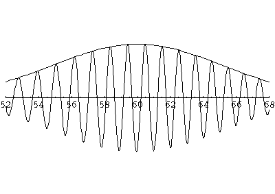
Here are some pictures of a k0=6, =1.5
wavefunction at various times.
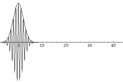
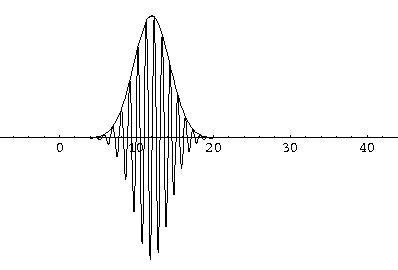
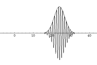
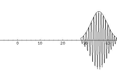
Notice that the central part of the wave packet moved from y=0,12,24,36 as t=0,1,2,3, that is to say that the "velocity" of the packet is about 12=2k0. Also notice that, as expected, the packet has expanded slightly.
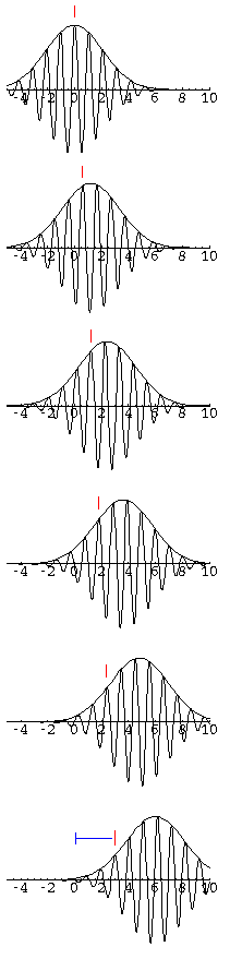
Notice that within the lump of probability you can see the
waves of the real part of . In the following sequence
of stills (for t=0, 0.1, 0.2, 0.3, ...), we follow one of these peaks
in Re() within the wave-packet. Notice that
this particular peak (marked in red) falls behind the wave-packet.
During the 1/2 tic time period displayed, the wave-packet as a
whole has moved forward 6 units, whereas the individual peak
has moved forward 3 units. The speed of an individual peak
is called the phase velocity; the speed of the wave-packet is called
the group velocity. For a free particle in QM the phase velocity is half the
group velocity.
All of these features can be seen in greater detail by examining the following QuickTime movie (4 Mb) on a frame-by-frame basis.
It is also interesting to view the moving wave in a frame that moves with the wave, as in this QuickTime movie (4 Mb).
Finally, I have stated that we can attribute the spreading of the
wave-packet to the different velocities that make up the packet. Classically
you should expect that the faster aspects of the wave-packet should
eventually move ahead of the slower. Thus since de Broglie's relationship associates
the local wavelength with the particle's momentum, we might expect that
the local wavelength at the front of the packet becomes shorter
than the local wavelength at the rear of the wave-packet. In our examples
we have chosen to minimize the velocity
differences, so the effect is small. Nevertheless, careful examination
of this t'=5 frame shows that the local wavelength at the front of this wave
is smaller than the wavelength at the rear of the wave: